LSTMs and HMMs to predict lithium-ion battery lifetimes

Introduction

Background and motivation

The rapidly increasing use of fossil fuels and its associated environmental costs has led to a growing need for efficient methods of energy storage. One widespread and readily available energy storage solution is the lithium-ion rechargeable battery, which is universally used as it has high energy storage capacity, high energy density, long lifetime, and relatively low environmental impact. They are commonly used in small electronics, including laptop computers, mobile phones, and power tools. More recently, as battery technologies have improved, they have been employed in electric and hybrid vehicles as well.

One problem inherent in these batteries is the mechanical strain which occurs as lithium ions travel from the cathode to the anode as part of normal battery operation. This can result in a buildup of cracks and charge heterogeneity inside the battery, which eventually contributes to a decrease of the battery’s energy capacity over many charge and discharge cycles. These effects, among others, contribute to a loss of a battery’s efficiency over time.

For practical purposes, battery failure is considered to occur when its capacity (i.e., the amount of charge it can hold) drops below a certain threshold value. When this happens, its power output drops and becomes unpredictable; this makes the battery much less efficient and potentially unsafe to use. There are several methods in practice which predict when a battery will fail. The prediction metric we will use is remaining useful life (RUL), which is defined at any time as the estimated number of cycles until the battery’s capacity drops below the threshold value.

There are several existing RUL prediction methods in use, falling into two categories: model-based and data-based models. The former relies heavily on a mathematical model specific to a battery, but is often prone to overfitting and is generally not able to take into account long-term performance and behavior of the battery. The latter class of RUL prediction methods uses machine learning techniques in order to model battery degredation without the use of complex mathematical models. In the past, methods including SVM and LSTM have been used with varying degrees of success. Zhang et al. (2017) employed an LSTM model in a similar fashion as the current study and showed that recurrent neural network (RNN) methods such as LSTM tend to show greater levels of accuracy with battery degredation, which is modeled naturally as sets of time-series data. We will focus on data-based models.

In this study, we will compare the performance of long short-term memory (LSTM) models and hidden Markov models (HMM) as RUL predictors. Both models have been applied successfully to time-dependent data in the past. Zhang et al. describe how LSTM is applied successfully to battery degredation data as time series of the battery capacity over cycles.

LSTM is a type of recurrent neural network which relies on specialized LSTM neurons.

Source: Wikipedia, Long short-term memory

The LSTM cell comprises an input gate, an output gate, and a forget gate, which control the flow of information through the cell. The input gate controls how much new information enters the cell, the forget gate controls how long information remains in the cell, and the output gate controls how much information leaves the cell via an activation function. Using an algorithm such as gradient descent and backpropagation, the parameters of these gates can be calculated and each cell can be tuned to use varying amounts of past data.

HMM is a discrete-time statistical model which assigns states to each point in time and attempts to calculate the conditional probability of transitioning into the next state at each time interval. If $X$ is a process with unobservable states and $Y$ is an observable process whose observed states we wish to use to make inferences about $X$, then the pair $(X, Y)$ is a hidden Markov model if for all $n$ in our time domain we have that

$$P(Y_n \mid X_1 = x_1, \dots, X_n = x_n) = P(Y_n \mid X_n = x_n).$$

In other words, we assume that the process $X$ depends only on the most recent state and not on any prior states. Typical HMM learning methods include various expectation-maximization algorithms employing maximum likelihood estimation.

In this case of battery failure, we assume the final state is absorbing - that is, once a battery is observed in this final state, it cannot enter a different state. This means that a battery that has failed cannot “un-fail.” This assumption allows the calculation of expected number of charge/discharge cycles until failure. In a Markov model with an absorbing state, the expected number of steps until absorption can be calculated as

$$t = (\mathbf{Q}-I)^{-1}\mathbf{c}$$

Here, $\mathbf{Q}$ is the square submatrix of the transition matrix of the Markov model that does not include the row or column of the absorbing state, and $\mathbf{c}$ is a column vector of all ones. This calculation is used to predict the remaining useful life of a battery. As the model categorizes batteries into the different states in the model, these categorizations can be used to determine the expected number of cycles until absorption, which signifies failure of the battery.

The critical difference between LSTM models and HMMs is the Markov assumption which is made in HMMs - that is, when working with a HMM, we assume that the underlying hidden process depends only on its current state and not any prior states. LSTM models, in contrast, are able to take into account past data and use this to make a future prediction. Thus, comparison of these two methods will reveal some information about the behavior of the processes underlying degredation of lithium-ion batteries.

For this study we use a dataset whose testbed comprises several 18650 sized rechargeable lithium-ion batteries who were run through charge, discharge, and electrochemical impedance spectroscopy cycles until failure, which is defined as a 30% reduction in the batteries’ nominal capacity of 2.0 amp-hours (Ah). In other words, we consider the batteries to have failed once their capacity reaches 1.4 Ah. We focus only on discharge cycles and consider the battery capacity vs. cycle as the time-series data with which we will train a LSTM model and a HMM.

Dataset

For our data, we used NASA’s publicly accessible repository of Lithium Ion Aging Datasets. These data were collected from a testbed at the NASA Ames Prognostics Center of Excellence (PCoE). A set of four Li-ion batteries were run through 3 different operational profiles (charge, discharge and impedance) at room temperature.

Charging was carried out in a constant current (CC) mode at 1.5A until the battery voltage reached 4.2V and then continued in a constant voltage (CV) mode until the charge current dropped to 20mA.

Discharge was carried out at a constant current (CC) level of 2A until the battery voltage fell to 2.7V, 2.5V, 2.2V and 2.5V for batteries 5 6 7 and 18 respectively.

Impedance measurement was carried out through an electrochemical impedance spectroscopy frequency sweep from 0.1Hz to 5kHz.

Repeated charge and discharge cycles result in accelerated aging of the batteries while impedance measurements provide insight into the internal battery parameters that change as aging progresses. The experiments were stopped when the batteries reached end-of-life (EOL) criteria, which was a 30% fade in rated capacity (from 2Ahr to 1.4Ahr).

Initially, we looked at the Impedance cycle to see if we could discern any kind of pattern that would suggest the age of the batteries. However, after some discussion, we decided to use the discharge cycle instead.

To clean and prepare the data for consumption by our LSTM and HMM code (written in python), we had to convert the MATLAB data files into csv files.

To do this we wrote MATLAB scripts to traverse the data structures and extract the data we required. We found that most of the data was already pretty clean except for some areas where initial readings were abnormal or non-existent. We removed the ones that were anomalous.

csv files of batteries (discharge and impedance)

B0005 discharge
B0005 impedance
B0006 discharge
B0006 impedance
B0007 discharge
B0007 impedance
B0018 discharge
B0018 impedance

Results

LSTM

Using LSTMS, we attempted to create a model that could learn from early capacity measurements (first 60% of cycles) of a single battery (0005) and effectively predict its remaining useful life. We developed two LSTM different models to this purpose.

Prediction of Capacity Reduction over Time with LSTM

In this model, we used the past capacity curve to predict the future capacity curve (over time). This was based on current literature in the field [Y Zhang et al]. We trained on 60% of the capacity data and used the resulting model to predict the curve for the remaining 40% of cycles. In order to train the LSTM, we modified the shape of the input data for supervised learning using time steps of 3 cycles. The i’th data item in our training data would have 3 features: capacity at cycle i, i-1, and i-2, and a truth value: capacity at cycle i+1. The model is used to predict a capacity for the next cycle, and this predicted value is iteratively fed back into the model to predict even further into the future. The point where the predicted curve hits 1.4 Ah is the predicted Remaining Useful Life. Our model contained an LSTM layer of 50 nodes followed by a dense layer of one node. We trained it for 600 epochs using the RMSProp optimizer. We found that adding anymore layers/nodes/epochs made the model susceptible to overtraining. Below, we show our result. Our model predicts an RUL of 106 while the real RUL is 124. RSME = 0.04 Ah

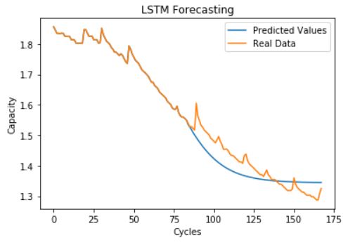
While this technique was very intuitive and supported by literature, it does not directly predict our desired goal: the Remaining Useful Life; instead, it predicts capacity. Therefore, we aren’t optimizing for the right RMSE (e.g. we optimize past models that predict RUL very well but have poor capacity RMSE). To fix this, we tried an alternative approach given below.

Direct Prediction of RUL over Time with LSTM

For this LSTM model, we used past capacity data to directly predict the RUL. We used a technique known as walk-forward validation. We train on all the capacity data up till the “current” cycle (in time steps of 3 cycles), and predict the RUL from the current cycle. Every time we “recieve” new data (move to the next cycle), we retrain on the new data and make a better prediction. Below is a graph of our predicted RUL at each cycle compared to the real value (starting from training on 60% of the cycles). For this model, we found that we benefitted from stacking an extra LSTM layer of 50 nodes and adding dropout layers. Dropout layers randomly remove a fraction (0.2) of the network nodes to prevent overfitting. We trained for 1000 epochs using the RMSProp optimizer and ran it till the failure point (RUL=0). RMSE = 11 cycles

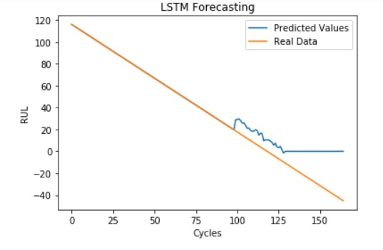
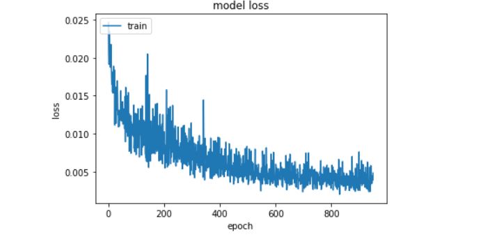
It is interesting to note that the model consistently errs at about +10 above the real RUL. This is probably because the model is overfitting to the small spikes in the capacity vs time curve and overestimating future capacity. Also, as expected, RUL prediction seems to get better as we get closer to the point of failure. Below we show our RMSE loss over training time.

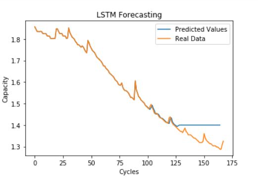
We also created a visualization where we used our predicted RUL at each cycle to calculate a predicted capacity for the consequent cycle as C_i+1 = C_i - (C_i - 1.4) / RUL. We ran this till the failure point.

Its important to note that this visualization seems to do much better than the first model only because it is predicting only one cycle into the future.

HMM

Seven HMM models were trained, with numbers of initial components ranging from 3 to 10. 10 was selected as the maximum number of components as the average number of cycles until failure was around 100, and too many components would lead to overfitting of the data. Thus the square root of the number of cycles until failure was used as a maximum number of components. Like the LSTM, HMMs were trained on capacity data per charge/discharge cycle. Data was split 75-25 between training and testing sets. Each model was trained four times in order to ensure convergence to the best local minima, and the model with the smallest root mean square error (RMSE) when tested on the testing data set was selected as the best performing model for that number of compartments.

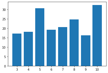
In this figure, the RMSE of the best performing model versus the number of initial components can be seen. The data generally shows an upward trend in the error as the number of components increases, likely due to the increase in number of learnable parameters as the number of components increases. Interestingly, the RMSE dropped dramatically to its lowest value with 9 components.

Here, we show the results of the prediction on the test data from the best overall model, with 9 initial components.

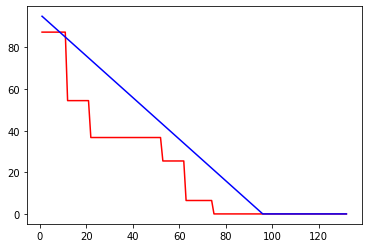
Here, remaining cycles until failure is plotted versus cycle number. The actual data is in blue and the predicted data is in red. It is apparent that this model tends to underpredict the number of cycles until failure, giving a low estimate of remaining useful life of the battery. Also of note is the number of steps in the predicted data. As the model was initialized with nine compartments, it is expected that the prediction data would have nine steps. However, upon visual inspection, only six discrete steps are present. The rest of the plots can be seen here:

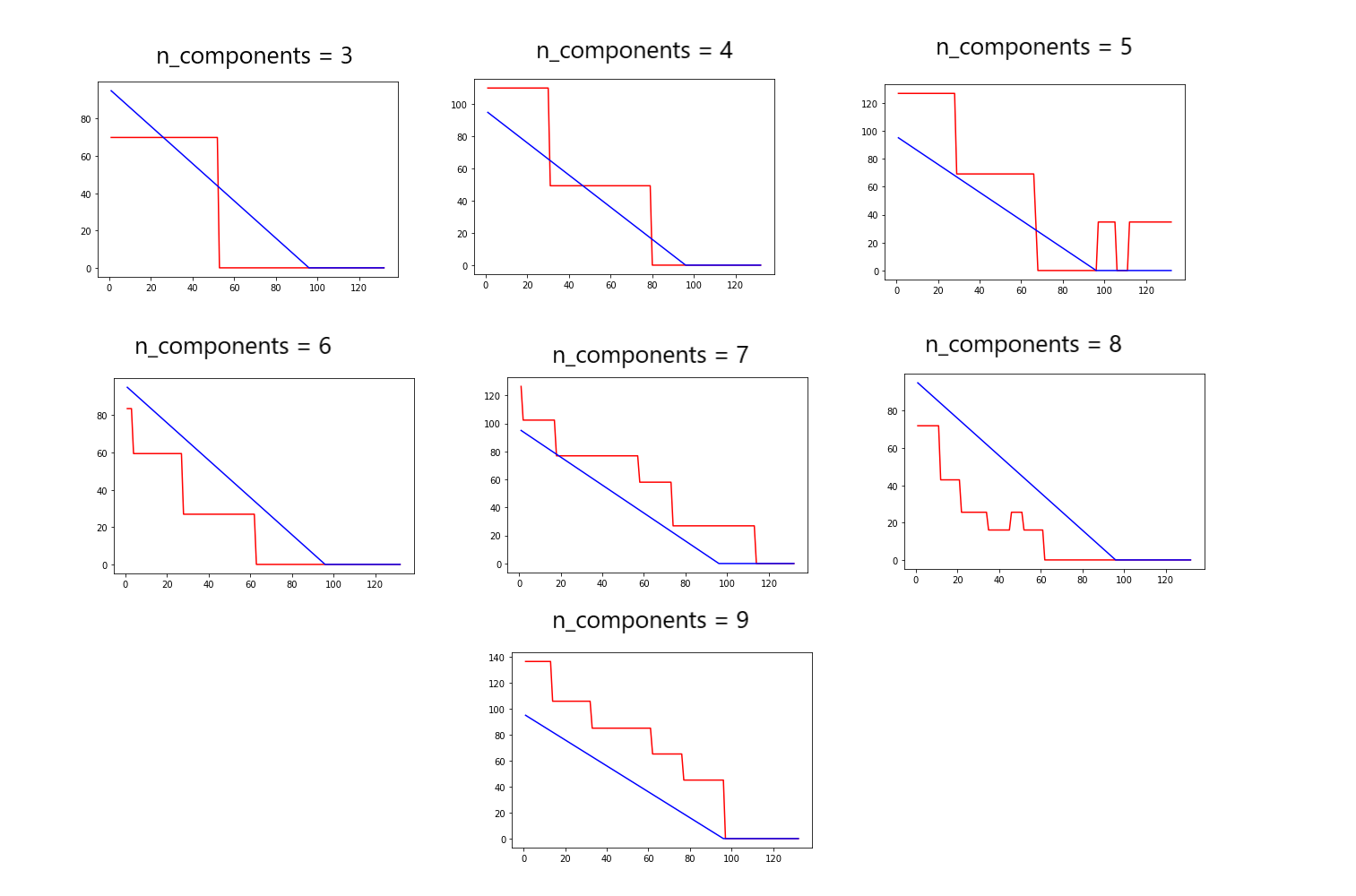
As seen in these figures, this behavior is consistent across all models. Each model has converged to a number of compartments smaller than the initial number. The most common number of compartments after convergence is six. This is consistent with the observation that the best performing model converged to six compartments.

Conclusion

Comparison of models

The two models applied to the data (LSTM and HMM) delivered differing levels of success modeling the data. The LSTM was accurate, but also generally susceptible to overtraining. It also allowed direct prediction of the RUL up to an accuracy of +/-10 cycles. The HMM, fitted into less than ten compartments, had an unpredictable accuracy as the number of compartments proved to be an unrelated hyperparameter. The predictions of the HMM were low in value as the predictions were discrete. The LSTM, with continuous predictions, was able to make more accurate predictions. The lowest RMSE of the LSTM was much lower than the lowest RMSE of the HMM.

While the LSTM was largely more successful than the HMM, the HMM was significantly more efficient. The first LSTM model was more efficient but less accuraet than the second LSTM model, which utilized walk-forward validation and had to be retrained every transition between cycles.

Though the LSTM model showed the most relevant predictions, these models are not ready for production without more training on larger data sets.

Further work

There are many possible directions that could be explored with regards to time-series RUL prediction. Convolutional neural networks (CNNs) are one promising avenue of study, as they have been successfully applied to time-series datasets in the past. CNNs operate by using a kernel to perform a convolution operation in a hidden layer instead of the usual matrix multiplication. Essentially, this abstracts the input data to a feature map in a different space.

Other methods that have seen success with time-series data are random forest, gradient boosting regressor, and time-delay neural networks. Additionally, it might be interesting to examine how simpler methods like polynomial or SVM regression compare to more complex neural-network based models.

In summary, there are many machine learning frameworks that could be useful with time-series data, and future work could compare these with the methods explored in this study.

References

Y. Zhang, R. Xiong, H. He and Z. Liu, “A LSTM-RNN method for the lithuim-ion battery remaining useful life prediction,” 2017 Prognostics and System Health Management Conference (PHM-Harbin), Harbin, 2017, pp. 1-4, doi: 10.1109/PHM.2017.8079316.

Credits

The data was cleaned by Luca and Daniel, the HMM model was created by Frank and Angad, and the LSTM model was created by Joel.